Introduction
The manifold hypothesis says that most real-world datasets lie approximately on a low-dimensional manifold, but by some Kantian twist of fate we rarely have direct access to this manifold1. As a result, most machine learning techniques utilize only local structure (e.g. the “loss + SGD” machine).
In contrast, Topological and Geometric Data Analysis (TGDA) is a burgeoning field that studies the global structure of data. This is exciting not only because of potential domain applications – it also opens possibilities for porting a lot of powerful and beautiful math to the ML realm.
One aspect of TGDA is non-Euclidean representation learning. In this post I discuss hyperbolic learning, a research area that has been very active in recent years. After introducing hyperbolic space and its connection to trees, I go over some developments in combinatorial methods for hyperbolic embeddings. At the end, I produce some example embeddings using Hyperlib.
Hyperbolic Space
I usually find it difficult to explain hyperbolic space to the geometrically uninitiated (it generally involves me going on about Riemannian metrics and curvature tensors while gesturing wildly at Escher’s Circle Limit). The geometry of a sphere or plane is easy to grasp, but negative curvature is unintuitive to our Euclidean brains.

Luckily, I can explain it simply if you know what a tree is: hyperbolic space is a continuous version of a tree.
To see what this means I have to introduce a notion of hyperbolicity invented by the great mathematician Gromov, which he originally used in the context of geometric group theory.
\(\delta\)-Hyperbolicity
Suppse \( X \) is a set of points and \(d(\cdot, \cdot)\) is a metric on \(X\) (a symmetric distance function that satisfies the triangle inequality).
Define the “Gromov product” as
$$ (x | y)_z = \frac{1}{2}(d(x,z)+d(y,z)-d(x,y)) $$
Roughly, the Gromov product measures the distance of \(z\) from the shortest path (the geodesic) connecting \(x\) and \(y\).
Definition: A metric space \( (X, d)\) is \(\delta\)-hyperbolic ( \(\delta \ge 0\) ) if
$$ (x | y)_w \ge \min( (x|z)_w, (y|z)_w) - \delta \quad \text{for all } x,y,z,w \in X.$$
This condition essentially says that no point in the triangle formed by \(x,y,z\) can be too far from one of the edges. In fact, it’s equivalent to require all triangles in \(X\) to be “slim”2, where \( \delta \) is the “slimness” parameter.
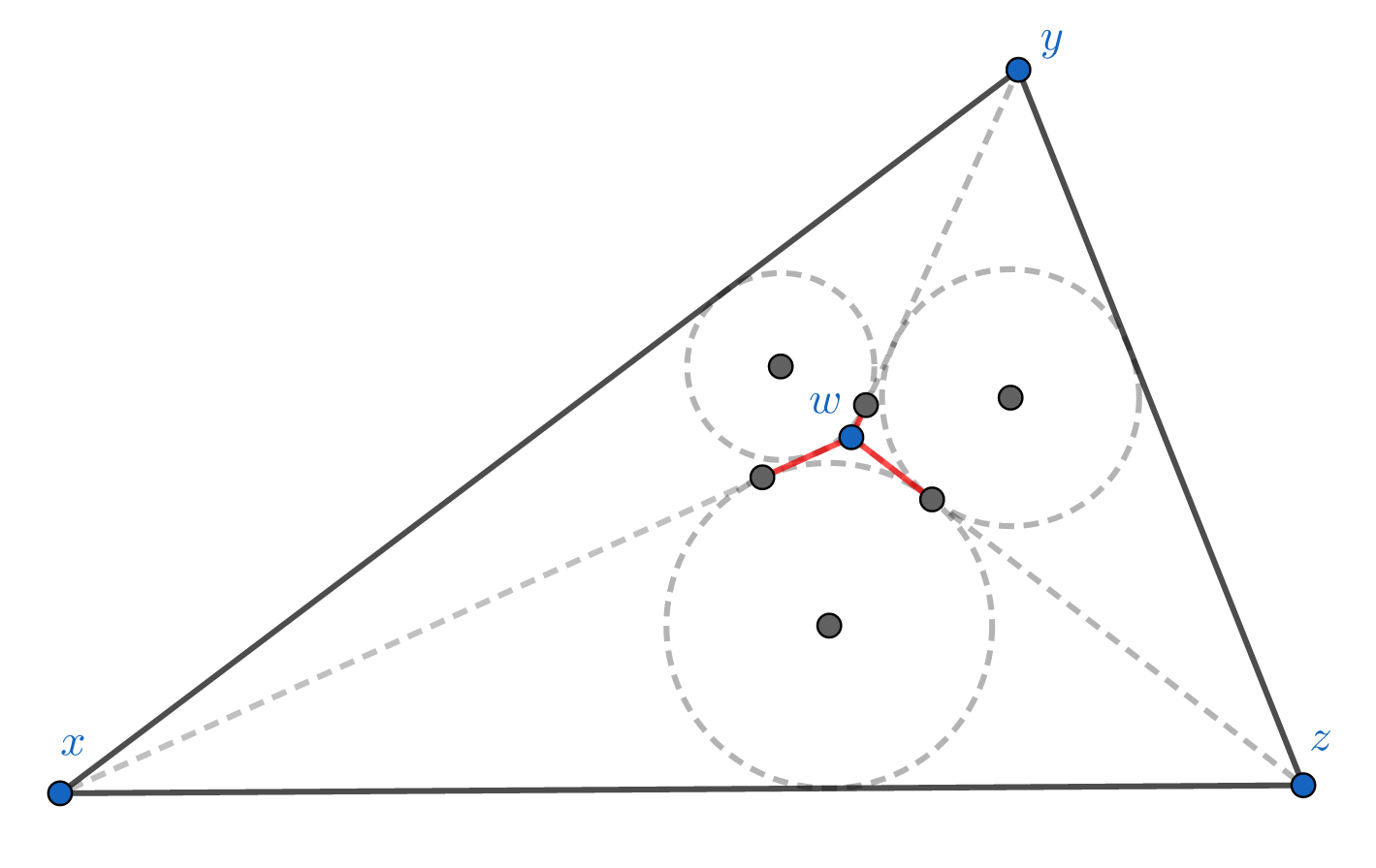
The delta-hyperbolic condition in the Euclidean plane. The diagram shows incircles of the triangles xyw, xwz, and zyw. The length of the 3 red segments equal to the 3 Gromov products
What kind of space has slim triangles (small \(\delta\))? A tree!
For example, take an unweighted tree with its shortest-path distance.
As a metric space it is 0-hyperbolic, i.e. \( (x|y)_w \ge \min( (y|z)_w, (z|x)_w ) \)
(Proof: Exercise).

A tree has no cycles, so every triangle is just a path – a degenerate triangle. Trees are therefore the most hyperbolic of spaces; 0-hyperbolic metrics are called tree metrics (note however not all tree metrics come from a tree graph).
Now it’s easy to imagine graphs with a small \(\delta\): they’re the “tree-like” ones with few long cycles.
Poincaré Disk Model
Graphs are well and good for you discrete-ophiles, but we want continuous hyperbolic spaces with derivatives and stuff!
There are many models of hyperbolic space3, but one of the easiest to visualize is the Poincaré model.
In 2 dimensions, it is the set of points in the Euclidean disk
\( \mathbb{H}^2 = \{ x\in \mathbb{R}^2 : |x| < 1 \} \) with the metric given by
$$ d_H(x,y) = \cosh^{-1} \left(1 + 2\frac{|x-y|^2}{(1-|x|^2)(1-|y|^2)}\right).$$
Nevermind where this crazy function comes from, just note that the distance gets huge near the boundary circle \( |x| \to 1 \) ( \( \cosh^{-1}(r) \sim \log(r) \) grows logarithmically ).
Geodesics (shortest paths) in this model are arcs of circles that intersect the boundary circle at right angles. As a result, triangles look like this:

To our Euclidean eyes, the triangles get smaller and more distorted towards the boundary, but all of these triangles are acutally the same size when measured with the Poincaré metric. Space expands exponentially near the boundary unlike Euclidean space, which may give you an idea of why it is like a tree.
As you might suspect, triangles in the Poincaré disk are “slim,” and it turns out this metric space is \(\delta\)-hyperbolic with \(\delta = \log(1+\sqrt{2}) \approx 0.881 \). This model can be generalized easily to higher dimensions, and lower or higher \(\delta\). Other common models of hyperbolic space are the Lorentz model (or hyperboloid model) and the upper-halfspace model.
I could go on for pages about hyperbolic space and its strange properties – I refer the interested reader to one of the many good introductory articles.
Hyperbolic Data
Now that we’ve established a correspondence “hyperbolic” ⟷ “treelike,” you may be wondering what type of data is hyperbolic.
The answer is: anything with a hierarchical structure. Words, social networks, the Internet, knowledge graphs, genomic data, images, even financial data – and that’s only the tip of the iceberg (see [5,6,8,9,10,11] and the references therein).
One way to understand the hyperbolic structure of these data is in terms of categorization (or hierarchical clustering for you ML people). Often there is a hierarchy of categories that gives rise to an underlying tree (Henri is a human; a human is a primate). However, we may get something that is only approximately a tree due to heterogenous or overlapping categories (Henri is a human; Henri is a mathematician; a mathematician is a human).
We therefore might expect many datasets to have a \( \delta \)-hyperbolic metric (this is indeed the case, and we can measure \( \delta \) directly). This leads to the idea of embedding data in hyperbolic space.
The Embedding Problem
The problem is now an algorithmic one: given data, compute a hyperbolic representation. A large portion of hyperbolic learning research focuses on this problem.
For data with a natural metric, it can be formulated as follows: given data \(X \) with a metric \( d \) find an embedding \(f: (X,d) \to (\mathbb{H}, d_H) \) where \( (\mathbb{H}, d_H ) \) is a model of hyperbolic space. The embedding should have “low distortion” by some measure; a common choice is the average distortion, defined by
$$D_{avg} = \frac{1}{\binom{n}{2}} \sum_{x,y\in X} \frac{|d_H(f(x),f(y)) - d(x,y)|}{d(x,y)}$$
where the sum is over distinct pairs \( \{x,y\} \) and \(n\) is the number of points in \(X\). Another measure is the worst-case distortion, defined by ratio of the maximum “stretch” \(d_H(f(x),f(y)) / d(x,y)\) to the minimum stretch. If one only cares about preserving neighborhoods (i.e. Voronoi cells) then a different measure called the mean average precision is used.
There are two main strategies to find an embedding:
- (SGD) Use a loss function and gradient descent to learn the embedding
- (Combinatorial) Embed the data into a (weighted) tree, then embed the tree in hyperbolic space
The SGD strategy for hyperbolic embeddings was pioneered by Nickel & Kiela [3,4], who demonstrated that datasets like WordNet can be embedded in hyperbolic space with low distortion and in low dimensions. The drawback of the SGD stategy is the computational cost and numerical instability of doing gradient descent with the Riemannian gradient (this is a problem for hyperbolic deep learning in general).
For the remainder of this post I’ll primarily talk about the combinatorial strategy.
Get in the Tree!
The second part of combinatorial strategy (embed a tree in hyperbolic space) is easy. An algorithm by Sarkar [2] embeds a tree with \(n\) nodes in the Poincaré disk in \( O(n) \) time. It guarantees that the worst-case distortion is at most \( 1+\epsilon \) if the edge weights are scaled appropriately (by contrast, a tree with constant branching factor – or more generally an expander graph – cannot be embedded with constant distortion in Euclidean space of any dimension).
The idea of Sarkar’s algorithm is simple: place a node at the origin and place all its children equally spaced in a circle around it. Then move one of the children to the origin (by a hyperbolic reflection) and repeat.
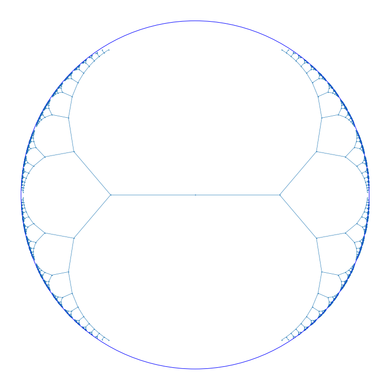
Here’s an example of an embedding of a complete binary tree in the Poincaré disk that achieves an average distortion of 0.153:
The authors of [1] provided a generalization of Sarkar’s algorithm to higher dimensions. The only downside of Sarkar’s algorithm is it requires high precision float arithmetic (as the points tend to the boundary).
Now we can address the first part of the combinatorial strategy (embed the data into a tree), which is the more interesting problem.
Many of the algorithms start from the following construction:
For three points \(x,y,z \in X\) form a tree by adding a new point \(t\) and edges \( ( t,x), (t,y), (t,z)\). In order to stay consistent with the original metric on \(X\), you’ll find that the edge weights have to be
$$ \begin{aligned} d(t,x) &= (y|z)_x\cr d(t,y) &= (x|z)_y\cr d(t,z) &= (x|y)_z. \end{aligned} $$
\(t\) is called a Steiner node and the 4-node tree is sometimes called a Steiner tree. Following the previous discussion, it may be interpreted as a category or cluster, depending on the data.
To illustrate this, suppose \(d(x,y) = d(y,z) = d(z,x) = 1 \). To form the Steiner tree we add a Steiner node at a distance 1/2 from \(x,y,\) and \(z\).

A relatively old algorithm that uses this idea is Neighbor Joining, which is typically used in bioinformatics for constructing phylogenetic trees from some measure of genetic distance between species. Abraham et al. [12] improved the construction and obtained precise bounds on the worst-case distortion for tree-like metric spaces4.
Recently, Sonthalia & Gilbert [7] introduced an algorithm called TreeRep to construct a tree from a \(\delta\)-hyperbolic metric. The idea is to start with the Steiner tree on \(x,y,z,t\) as above, sort the remaining points into zones based on their distance to the Steiner tree, then recursively add them to the tree.
TreeRep reconstructs 0-hyperbolic metrics perfectly, but there is unfortunately no distortion bound for \(\delta > 0\). However, empirically TreeRep outperforms other combinatorial methods (as well SGD methods) on both speed and distortion.
Variations on these ideas are still inspiring new algorithms for hyperbolic embeddings (particularly interesting is [13] ).
Examples with Hyperlib
Finally, here are a couple examples of combinatorial embeddings using Hyperlib, a library for hyperbolic learning I’m contributing to.
As I mentioned before, a classic application of tree embedding is the construction of phylogenetic trees. Sarich [14] measured the “immunological distance” between 8 species of mammals. Let’s embed them in hyperbolic space with TreeRep and Sarkar’s algorithm5.
import numpy as np
import networkx as nx
from hyperlib.embedding.graph import *

labels = {0:"dog", 1:"bear", 2:"raccoon", 3:"weasel",
          4:"seal", 5:"sea lion", 6:"cat", 7:"monkey"}
metric = np.array([
        32.,  48.,  51.,  50.,  48.,  98., 148.,
        26.,  34.,  29.,  33., 84., 136.,
        42.,  44.,  44.,  92., 152.,
        44.,  38.,  86., 142.,
        24.,  89., 142.,
        90., 142.,
        148.])

T = treerep(metric)
G = to_networkx(T) #convert to a nx.Graph
embed = sarkar_embedding(G, 12, tau=0.2, precision=80)
plot_embedding(G, emb, labels=labels)
Here’s the resulting tree:

The real evolutionary tree looks like this.
Here’s the code to plot the embedding:
import matplotlib.pyplot as plt
from matplot.collections import LineCollection

def plot_embedding(G, embedding, **kwargs):
    pts = np.array(list(map(float, embedding))).reshape(-1,2)
    size = kwargs.get("figsize", (15,15))
    plt.figure(figsize=size)
    labels = kwargs.get("labels", None)
    if labels:
        for i in labels:
            plt.annotate(labels[i], pts[i],
                         size=14,
                         bbox=dict(facecolor='grey',alpha=0.1))

    lines = [(pts[e[0]],pts[e[1]]) for e in G.edges]
    lc = LineCollection(lines,linewidths=0.7)
    circle = plt.Circle((0, 0), r, fill=False, color="b")
    plt.gca().add_artist(circle)
    plt.gca().set_aspect("equal")
    plt.xlim(-1.1, 1.1)
    plt.ylim(-1.1, 1.1)
    size = kwargs.get("node_size", 10)
    plt.scatter(pts[:,0],pts[:,1], s=size)
    plt.gca().add_collection(lc)
    plt.axis("off")
    plt.show()
For a bigger dataset, let’s look at the hyperlink graph for .edu sites, available here. Let’s also measure the \(\delta\) constant for the data and the average distortion of the embedding. Note that TreeRep is a randomized algorithm, so you can generate multiple trees and take the best one.
from scipy.sparse.csgraph import shortest_path
from scipy.spatial.distance import squareform
from hyperlib.embedding.metric import delta_rel

def distortion(tree, metric, n):
	'''Find the average distortion of the tree embedding for n points'''
	M = to_sparse(tree)
	tree_metric = squareform( shortest_path(M, directed=False)[:n,:n] )
	return np.mean( np.abs(tree_metric - metric) / metric )

adj_mat = sp.io.mmread("web-edu.mtx") # load adjacency matrix
metric = shortest_path(adj_mat) # compute the graph metric
delta_r = delta_rel(metric[:1000,:1000]) # estimate the relative delta constant
metric = squareform(metric)

# generate 10 embeddings
for _ in range(10):
	T = treerep(metric)
	print( distortion(T, metric, adj_mat.shape[0]) )
The best average distortion I got out of the 10 tries was 0.0492. The relative \(\delta\) (i.e. normalized by the maximum distance) is approximately 0.2.
Thanks for reading, stay tuned for more!
Interested in hyperbolic deep learning or want to contribute to Hyperlib?
Join us at nalex.ai! You can contact Nathan at nathan.francis@nalex.ai and Alex at alexander.joseph@nalex.ai.
References
[1] C. De Sa, A. Gu, C. Ré, F. Sala, Representation Tradeoffs for Hyperbolic Embeddings
[2] R. Sarkar, Low Distortion Delaunay Embedding of Trees in
Hyperbolic Plane
[3] M. Nickel & D. Kiela, Poincaré Embeddings for Learning Hierarchical Representations
[4] M. Nickel & D. Kiela, Learning Continuous Hierarchies in the Lorentz Model of Hyperbolic Geometry
[5] I. Chami, A. Wolf, D. Juan, F. Sala, S. Ravi, C. Ré, Low-Dimensional Hyperbolic Knowledge Graph Embeddings
[6] V. Khrulkov, L. Mirvakhabova, E. Ustinova, I. Oseledets, V. Lempitsky, Hyperbolic Image Embeddings
[7] R. Sonthalia, A. C. Gilbert, Tree! I am no Tree! I am a Low Dimensional Hyperbolic Embedding
[8] A. Tifrea, G. Bécigneul, O. Ganea, Poincaré GloVe: Hyperbolic Word Embeddings
[9] O. Ganea, G. Bécigneul, T. Hofmann, Hyperbolic Entailment Cones for Learning Hierarchical Embeddings
[10] D. Krioukov, F. Papadopoulos, M. Kitsak, A. Vahdat, M. Boguna, Hyperbolic Geometry of Complex Networks
[11] R. Sawhney, S. Agarwal, A. Wadhwa, R. R. Shah, Exploring the Scale-Free Nature of Stock Markets: Hyperbolic Graph Learning for Algorithmic Trading
[12] I. Abraham, M. Balakrishnan, F. Kuhn et al., Reconstructing Approximate Tree Metrics
[13] I. Chami, A. Gu, A. Chatziafratis, C. Ré, From Trees to Continuous Embeddings and Back: Hyperbolic Hierarchical Clustering
[14] V. Sarich, Pinniped Phylogeny
-
In some low-dimensional cases it is tractable. A notable experiment by Carlsson showed that 3x3 pixel patches on a dataset of black and white photos lay on a Klein bottle in \( \mathbb{R}^9 \) ↩︎
-
The definition of \(\delta\)-hyperbolic works for any metric space (which is a very general notion). For simplicity we can assume \(X\) has nice enough properties, like being a geodesic space. In that case, the “slimness” of geodesic triangles is indeed an equivalent definition (called the Rips condition). ↩︎
-
More specifically, by “hyperbolic space” I mean the (unique) complete \(n\)-dimensional Riemannian manifold with constant negative scalar curvature -1. Note that “hyperbolicity” as defined here can apply to any metric space, but most people will be thinking of the Riemannian manifold if you say “hyperbolic space.” ↩︎
-
They actually use a slightly different condition from \(\delta\)-hyperbolicity which they call the “\(\epsilon\) – 4 points condition.” This condition is invariant under scaling unlike \(\delta\)-hyperbolicity. The conditions coincide for \(\delta=\epsilon=0\). ↩︎
-
At the time of writing
sarkar_embeddingis only on this fork of Hyperlib. ↩︎