“There is geometry in the humming of the strings, there is music in the spacing of the spheres.”
– Pythagoras
Introduction
Recently I started exploring the world of error-correcting codes, and algebraic codes in particular. It’s a perfect example of mathematical hacking, where the Platonic realm of mathematical objects collides with the concrete world of signals, circuits, and CPUs to create something incredibly useful.
In this post I’ll share what I’ve learned so far about algebraic codes and go into some detail about Reed-Solomon and BCH codes. As a bonus I’ll show how to create QR codes.
Note on code examples: The full code for this post is at meiji163/ecc-clj. See the addendum on Clojure for how to play with it yourself.
Algebra Background
This section introduces some algebra needeed to understand algebraic codes. I’ve tried to make it understandable to those without an extensive math education. Feel free to skip ahead and come back later.
Finite Fields
A field is (roughly) a structure where you can add, subtract, multiply, and divide in the ways you’re used to. You’re already familiar with the field of real numbers, called \( \mathbb{R}\). You may also be familiar with the field of integers modulo p, called \(GF(p)\)1 (also known as \( \mathbb{Z}/p\mathbb{Z}\)). You add and multiply the same as regular integers, but take the remainder of the result when divided by \(p\).
For number-theoretic reasons2, \(p\) has to be a prime for division to work. This ensures that for all \(a = 1,2,\dots,p-1\) there is an integer \(0 < b < p\) such that
$$a \cdot b = 1 \pmod{p}.$$
So \(b\) is the inverse of \(a\). Division by \(a\) is then defined as multiplication by \(b.\)
As an example field, take the teeny little \(GF(2)\). It has two elements 0 and 1.
$$ \begin{aligned} 1 + 1 &= 0 \cr 1 + 0 &= 1 \cr 1 \cdot 1 &= 1 \cr 1 \cdot 0 &= 0 \end{aligned} $$
We could represent this in code as a collection of the field operations
(def GF2
  {:+ bit-xor
   :- bit-xor
   :* bit-and
   :/ bit-and})
You may think, “You have shown me one example of a finite field, now I demand a complete classification of all finite fields!"
Luckily, it can be shown3 that the number of elements a finite field can have must be \(p^n\) for some prime \(p\) and some integer \(n \gt 0\). We have seen the ones with \(p\) elements, in the next section we’ll see the other ones.
Polynomial Fields
Whenever you have a field \(F\), you can create polynomials whose coefficients are elements of \(F\). It’s usually called \(F[x]\)4. For example, a polynomial with binary coefficients like \(x^3 + x + 1\) is a member of \(GF(2)[x]\) .
Polynomials are a bit like vectors. Think of the coefficient of \(x^n\) as the value in the nth slot of a vector, e.g.
$$ 1x^0 + 1x^1 + 0x^2 + 1x^3 \leftrightarrow (1,1,0,1).$$
Now to add polynomials, we just add each corresponding coordinate of the vectors.
So then polynomial multiplication also defines multiplication of vectors?
Not quite. The trouble is when you multiply two polynomials, the degree of the product polynomial is can grow without bound! That’s not good if we want the vector size to be fixed.
This is where we take inspiration from the integers mod \(p\). In that case, whenever we get a result bigger than \(p\), we divide it by \(p\) and use the remainder instead. Similarly, for polynomials we choose a “modulus” polynomial \(p(x)\) with degree \(n\). Whenever a polynomial has a degree greater than \(n\), we divide it by \(p(x)\) and take the remainder polynomial. The reason this works is that, like the integers, polynomials have a Euclidean algorithm.
Can you use any modulus polynomial you want?
You can, but in general you get a “quotient ring” and not a field. Like the integer case, we have to choose \(p(x)\) to be “prime” in order to make division work. As you might guess, a prime polynomial is one that can’t be factored into other polynomials – remarkable how similar polynomials and integers are!
Constructing \(GF(2^n)\)
To see this in action let’s construct \(GF(2^3)\) from \(GF(2)\) polynomials.
Let \(p(x) = x^3 + x + 1\), which is a prime polynomial over \(GF(2)\). Now the distinct nonzero elements of the field are the eight \(GF(2)\) polynomials with degree < 3. We can multiply them like so
$$ \begin{aligned} x \cdot (x^2 + x) = x^3 + x^2 = x^2 + x + 1 \end{aligned} $$
where we replaced \(x^3\) by \( x + 1\), or equivalently, divided out \(p(x)\).
When the polynomials are as viewed binary vectors, we can interpret each vector as spelling out an integer in binary. For example \(x^2 + x + 1 \leftrightarrow 111_2 = 7\). Each field element gets assigned a number 0-7 according to this notational pun. But beware, you can’t add and multiply them like regular integers5!
Yet another way of representing finite fields comes from the primitive element theorem, which says that every finite field has a special element \(\omega\), called the primitive element, such that the successive powers \(\omega^1, \omega^2, \dots \) generate the whole field.
In our contruction of \(GF(2^3)\), a primitive element is the polynomial \(x\), aka “\(2\)” in our binary labeling scheme. Compare the different representations in the table below.
| decimal | binary | polynomial | exponential |
|---|---|---|---|
| 2 | 010 | \(x\) | \( \omega^1\) |
| 4 | 100 | \(x^2\) | \( \omega^2\) |
| 3 | 011 | \(x+1\) | \( \omega^3\) |
| 6 | 110 | \(x^2+x\) | \( \omega^4\) |
| 7 | 111 | \(x^2+x+1\) | \( \omega^5\) |
| 5 | 101 | \(x^2+1\) | \( \omega^6\) |
| 1 | 001 | \(1\) | \( \omega^0 ( = \omega^7 )\) |
We can implement this construction in code with something like this
(defn char2-field
  "construct field GF2[x]/<p(x)>
  given a primitive element and generating polynomial"
  [prim poly]
  (let [invs (char2-invs prim poly)
        n-elts (bit-shift-left 1 (bindeg poly))
        exp (vec (take n-elts
                   (iterate #(binmod (bin* % prim) poly) 1)))]
    {:unit 1
     :zero 0
     :primitive prim
     :inv invs
     :exp exp
     :+ bit-xor
     :- bit-xor
     :* (fn [p1 p2] (binmod (bin* p1 p2) poly))
     :/ (fn [p1 p2] (binmod (bin* p1 (invs p2))))}
    ))
The important points are that exp is a vector containing \(\omega^0, \omega^1, \dots, \omega^{2^n - 1}\),
and we define the field multiplication :* and field :/ with the functions binmod and bin* that implement GF2-polynomial modulo reduction and multiplication, respectively.
Now we can create GF8!
(def GF8
  "GF(8) constructed as GF2[x]/<x^3+x+1>"
  (let [GF2-poly (parse-bin "1011")]
    (char2-field 2 GF2-poly)))

;; examples
(let [mul (:* GF8)
      add (:+ GF8)
      div (:/ GF8)]
  (mul 3 3) ;; => 5
  (add 7 6) ;; => 1
  (div 5 4) ;; => 6
)
Error Correcting Codes
“Thus finding an error-correcting code is the same as finding a set of code points in the \(n\)-dimensional space which has the required minimum distance between legal messages”
– Richard Hamming, The Art of Doing Science and Engineering
The main problem motivating error correcting codes is reliable data transmission. When sending symbols (such as bits) over a medium that can introduce errors or erasures, how do you ensure that your intended message gets through?
Hamming’s insight was to formulate this as a max-min distance problem. Let’s consider the symbols as elements of a finite field \(F\). Then a block of \(n\) symbols, or “word”, corresponds to a vector in \(F^n\). What we want is a set of “codeword” vectors such that whenever errors occur, the erroneous vector can be mapped uniquely to the “closest” correct codeword vector.
Thus we need the codewords to be as “far apart” as possible, to minimize the chances of a word being “close” to two codewords simulatenously. The Hamming Distance, defined as the number of places where two words differ, is exactly the right notion of distance to measure this. Now the problem can be phrased as:
Find a set of codewords that maximizes the minimum distance betweeen any two codewords.
Equivalently, find a packing of non-intersecting spheres, such that the smallest radius is as large as possible.
Algebraic Codes
Codeword vectors can be chosen arbitrarily, but to make the problem tractable we impose an algebraic structure on the codewords, like a musician might impose meter and harmony on their music.
First we require that the codewords form a linear subspace of \(F^n\). That means whenever we add two codeword vectors or scale a codeword vector, we get another codeword vector. These are called linear codes. It’s not too hard to bound the best possible minimum distance for linear codes.
But first, a little more terminology: A code that encodes length \(k\) words into length \(n\) codewords and uses \(n-k\) check symbols is called an \( (n, k)\) code. Now we can state the
Hamming Bound: The minimum distance \( d_{min} \) between any two codewords of a \( (n,k) \) linear code satisfies \(d_{min} \le n-k+1\).6
This tells us the max number of errors a linear code can correct is \( \lfloor (n-k)/2 \rfloor \). However it does not tell us if such a code exists for a given \(n\) and \(k\) (booo!).
Example: The \( (7,4) \) binary Hamming code can correct 1 error. Its codewords form a four-dimensional subspace of \(GF(2)^7\) spanned by these vectors:
$$ \begin{aligned} 1000110 & \cr 0100101 & \cr 0010011 & \cr 0001111 \end{aligned} $$
What’s with the vectors and linear subspaces? I was promised polynomials!
But remember polynomials are like vectors too – we view the coefficients as vector coordinates. Then we can use a “generator polynomial” \(g(x)\) with degree \(n-k\) to generate a linear code as follows.
For every “word polynomial” \(w(x)\) of degree \(k\), the product \(g(x)w(x)\) defines a codeword polynomial of degree \(n\). Considered as vectors, these polynomials span a linear subspace of \(F^n.\) For example, \(g(x) = x^3+x+1\) generates the Hamming code above.
Cyclic Codes
Linear codes are great, but can we impose even more structure to find better codes? One idea is to consider linear subspaces that are highly symmetrical. That is where cyclic codes come in.
A cyclic code is a linear code that is invariant under a cyclic shift, e.g. if 1100 is a codeword then so is 0110 and 0011. If we translate this back to polynomial language, it requires that \(x^n\) “wraps around” and becomes \(x^0\). Algebraically, this means we take the ring of polynomials \(F[x]\) modulo \(x^n-1\)7. However we say it, what it means in practice is that we carefully choose the generating polynomial \(g(x)\) to be a factor of \(x^n-1\).
Example: Here are some factorizations of \(x^n-1\) over \(GF(2)\) into prime polynomials.
| \(n\) | Factorization of \(x^n - 1\) |
|---|---|
| 3 | \( (1+x)(1+x+x^2) \) |
| 5 | \( (1+x)(1+x+x^2+x^3+x^4)\) |
| 7 | \( (1+x)(1+x^2+x^3)(1+x+x^3)\) |
| 9 | \( (1+x)(1+x+x^2)(1+x^3+x^6)\) |
For each \(n\), a choice of factors gives you a cyclic code. For example choosing \(g(x) = 1+x\) gives you a simple code that adds one parity-check bit.
It’s fun to discover what codes these polynomials will produce, but it’s usually not easy to see what the minimum distance is. For that we need to use more strategic constructions.
(An aside for true math nerds: let me mention a “platypus” of the cyclic code zoo. The \((23,12)\) binary Golay code has a minimum distance of 7 and perfectly partitions the space \(GF(2)^{23}\) into spheres of radius 3. Its automorphism group is a sporadic group. The derivative \((24,12)\) Golay code is even more amazing and bizzare8.)
Reed-Solomon Codes
Reed-Solomon codes are some of the best and most widely used cyclic codes. To make your own \( (n,k) \) RS code, let \(\omega\) be a primitive element of your field \(F\). For the generating polynomial, cook up a polynomial in \(F[x]\) with roots at \(\omega^j, \omega^{j+1}, \dots, \omega^{j+m}\) for some integers \(j \ge 0\) and \(0<m<n\). For example,
$$ g(x) = (x-\omega)(x-\omega^2)\dots(x-\omega^m).$$
To guarantee this generates a cyclic code, we require that the size of the field \(F\) equals \(n\). Then \(g(x)\) is a factor of \(x^n - 1\) because \(\omega^n = 1\).
OK I cooked up my RS code, but why is it good?
It can be shown9 that whenever a \( (n,k) \) RS code exists, it achieves equality in the Hamming bound, i.e. \(d_{min} = n-k+1\). So these codes are optimally error correcting linear codes.
What accounts for this? It’s closely related to the Fourier transform over the field \(F\). If you’re familiar with the Discrete Fourier transform of a vector, it’s exactly the same except \(\omega\) plays the role of \(e^{-2\pi i/n}.\) Requiring \(\omega^j\) to be a root of \(g(x)\) is equivalent to requiring the \(j^{th}\) component of the Fourier transform to be zero.
The RS generating polynomial is then analogous to a low-pass frequency filter, which forces the frequencies of all codewords to be greater than some value. This forces the minimum weight (i.e. number of nonzero components) of a codeword to be bounded away from 0.
(This is a manifestation of the uncertainty principle, which roughly says that you cannot be simultaneously localized in both frequency and position. [8])
Examples: Let’s construct a \( (7,3) \) RS code over \( GF(8) \), using the representation of \(GF(8)\) from before. Let’s choose the generating polynomial as
$$ g(x) = (x-\omega^4)(x-\omega^5)(x-\omega^6)(x-\omega^7).$$
(def RS-7-3
  (reduce
   (fn [p1 p2] (p/* p1 p2 GF8))
   [[7 1] [6 1] [5 1] [1 1]]))
Now I can encode my favorite integer, 163.
With check symbols it is 3326163. Now I can change any two of the symbols and it decodes to 163.
(encode [1 6 3] RS-7-3 GF8) ;; => [3 3 2 6 1 6 3]
(RS-7-3-decode [3 3 2 6 1 6 3]) ;; => [1 6 3]
(RS-7-3-decode [1 3 2 6 1 7 3]) ;; => [1 6 3]
(RS-7-3-decode [3 3 2 6 6 6 6]) ;; => [1 6 3]
It feels magical when you see it up close!
For a bigger example, let’s construct a \( (255, 233) \) RS code over \(GF(256)\). It uses 32 check symbols to correct 16 errors (here the symbols are bytes). This code is one recommended by the “Consultative Committee for Space Data Systems” [4]. Famously, it was used for Voyager mission communications (in combination with other error-correcting codes).
(def RS-255-223
  (let [exp (:exp GF256)
        roots (for [e (range 1 33)] (exp e))]
    (reduce
     (fn [p1 p2] (p/* p1 p2 GF256))
     (for [r roots] [r 1]))))

;; example encoding
(let [message (str
       "Hello world! This is meiji163 transmitting from Neptune. "
       "It's cold here, Please send hot chocolate. Thanks. "
       "Now that I think of it, ramen would be good too if you have some.")
      data (map int message)
      padded (p/shift-right data (- 223 (count data)))]
      (encode padded RS-255-223 GF256))
BCH codes
Bose–Chaudhuri–Hocquenghem (BCH) codes follow a similar idea to Reed-Solomon codes. A limitation of RS codes is that the field has to be the same size as \(n\), the codeword length.
However it is still possible to specify the roots of \(g(x)\) in an extension field of \(F\). To see what I mean, let \(\omega = 2\) be a primitive element of \(GF(16)\) and let $$ \begin{aligned} g(x) &= (x-\omega)(x-\omega^2)(x-\omega^3)(x-\omega^4) \cr &= (x^4+x+1)(x^4+x^3+x^2+1). \end{aligned} $$
This polynomial has coefficients in \(GF(2)\), but its roots lie in the bigger field \(GF(16).\) This is analogous to a polynomial with real-valued coefficients having complex roots. The code generated by this polynomial is called the \((15,7)\) binary BCH code, which corrects 2 errors.
In general, we can construct a BCH code with minimum distance at least \(d\) by specifying a consecutive block of \(d-1\) zeros in an extension field.
Codecs
As I said above, given a generating polynomial \(g(x)\) and data polynomial \(w(x)\) one way to encode is to use \(g(x)w(x)\) as the codeword. The codeword polynomials are the ones divisible by \(g(x).\)
It’s convenient to use an encoding where the symbols of \(w(x)\) are visible in the codeword. To do this, set the top \(k\) coefficients as the coefficients of \(w(x)\), then add a degree \(n-k\) polynomial such that the codeword \(c(x)\) is divisible by \(g(x).\) Algebraically, \( c(x) = x^k w(x) + r(x) \) where \(r(x) = -x^k w(k) \pmod{g(x)}\).
(defn encode
  [data-poly gen-poly & [field]]
  (let [field (or field p/default-field)
        shifted (p/shift-right
                 data-poly (dec (count gen-poly)))
        rem (p/mod shifted gen-poly field)]
    (p/+ shifted rem field)))
Decoding is considerably harder because we have to exploit the algebraic structure of the code to locate the errors and their magnitudes. For small codes, you can make a table of error patterns and their remainders modulo \(g(x)\). For example,
(def RS-7-5-table
  "Decoding table for (7,5) Reed-Solomon code."
  (let [errors (single-errors 7 8)
        rems (map (fn [e] p/mod e RS-7-5 GF8) errors)]
    (zipmap rems errors)))
Given a message \(m(x)\) simply look up the error from \(m(x) \pmod{g(x)}\).
To decode larger RS codes the main tool is syndromes. Syndromes are defined as \(S_j = m(\omega^j)\) for all \(\omega^j\) that are specified as the roots of \(g(x)\). If no errors occured, all the syndromes will be zero.
On the other hand, if a correctable number of errors occurred, the idea is to form a linear system of equations using the syndromes to find the positions of the errors and the locations. I implemented the linear solver decoder here.
;; decoding (255,223) RS code
(let [err [0 42 1 0 0 163 0 0 66 0 0 0 0 0 101 100]
      max-errs 8
      decode-me (p/+ msg-poly err GF256)]
  (decode decode-me max-errs GF256)))
  ;; => {:locations [1 2 5 8 14 15],
  ;;     :sizes [42 1 163 66 101 100]}
A more efficient decoder is based on the Berlekamp-Massey algorithm, which I haven’t implemented. (Maybe you can, my brave reader)
Generating QR Codes
Typically error-correcting codecs are implemented in hardware circuits, which of course run several orders of magnitude faster than my implementation. Just to prove that my terribly slow implementation isn’t completely useless, I made a QR code generator.
There are many versions of QR codes, so I went with the 21x21 version as specified by the ISO/IEC standard [5]. I implemented just enough of the standard to make some example QR codes.
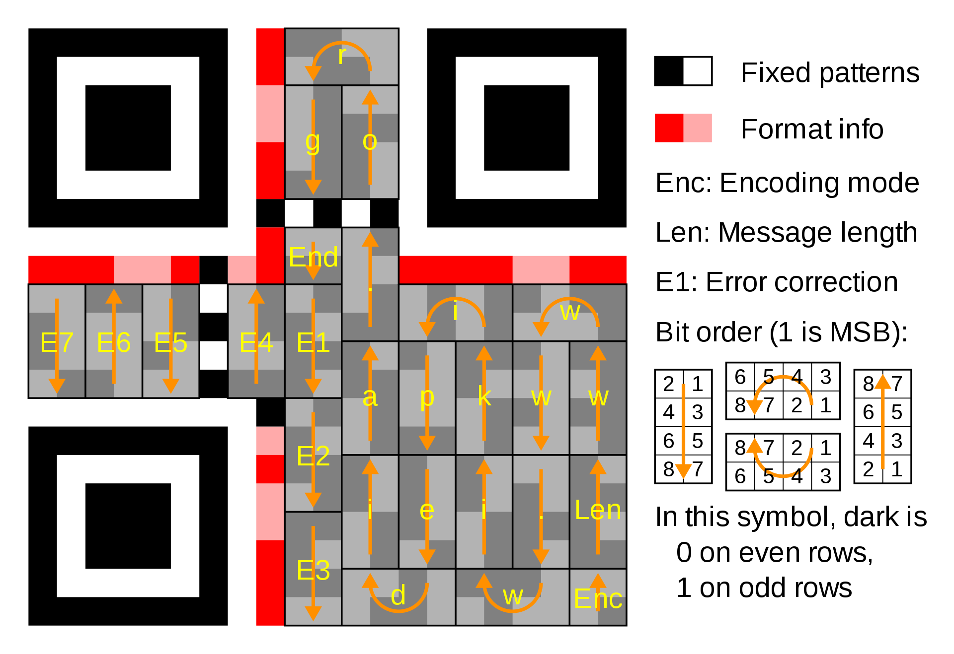
QR specification
There are two error-correcting codes involved in the QR code. One is for the “format bits” and the other is for the “data bits”.
Format bits: There are 5 format bits. The first 2 specify the error-correction level and the last 3 specify the bitmask. The 5 bits are protected by a \( (15,5) \) BCH code with 10 check bits. This can correct up to 3 errors. Two copies of the encoded bits are included, for a total of 30 bits.
Data bits:
The message can be up to 17 bytes.
The message bits are prepended with a 4-bit datatype code followed by an 8-bit integer specifying the message length. The 4-bit end sequence 0000 is appended to the message.
Finally, these 19 bytes are encoded with a \( (255, 248) \) Reed-Solomon code, which can correct 2 byte errors. It can detect (but not correct) 3 errors. You may see this code called a \( (26, 19) \) code because only 19 of the 248 bytes are used. This is the lowest error correcting level; other possible generating polynomials are listed in the standard.
Finally, the data bits are masked with a pattern specified in the format bits. The purpose of the bitmask is to preventing large areas of a single color.
The implementation of the RS and BCH codes is straightforward. We just have to be careful to use the same GF256 construction and generating polynomial as the one specified in the standard (Annex A in the manual).
The generating polynomial for the Reed-Solomon code is
$$ g(x) = 117 + 68x + 11x^2 + 164x^3 + 154x^4 + 122x^5 + 127x^6 + x^7 $$ which is computed from \((x-\omega^0)(x-\omega^1)\dots(x-\omega^6)\).
(def GF256
  "GF(256) constructed as GF2[x]/<x^8+x^4+x^3+x^2+1>"
  (let [GF2-poly (p/parse-bin "100011101")]
    (p/char2-field 2 GF2-poly)))

(def RS-255-248
  "(255,248) Reed-Solomon code over GF256"
  (let [roots (take 7 (:exp GF256))]
    (reduce
     (fn [p1 p2] (p/* p1 p2 GF256))
     (for [r roots] [r 1]))))
For the BCH code, the generating polynomial is the minimal polynomial of \(\omega, \omega^2, \dots, \omega^6\) over \(GF(2)\). This turns out as $$ (1+x+x^4)(1+x+x^2+x^3+x^4)(1+x+x^2). $$
(def BCH-15-5
  (reduce
   (fn [p1 p2] (p/* p1 p2 GF2))
   [[1 1 0 0 1] [1 1 1 1 1] [1 1 1]]))
Encoding the format bits:
(defn fmt-bits [mask]
  (let [mb [0 0 1]
        ec-level [0 1]
        bits (reverse (concat ec-level mb))
        enc-bt (ecc/encode bits ecc/BCH-15-5 ecc/GF2)]
    (p/+ (reverse enc-bt) fmt-bitmask ecc/GF2)))
I’ll omit encoding the data bits; it’s not as succinct because you have to move around many bits and pieces and pieces of bits. There are also some details with the bit ordering that bit me a few times (OK I’m done punning for a bit). Anyways the full code is here.
Now we can reproduce the QR code from the Wikipedia diagram above.
(let [mask-code 1
      databits (->> "www.wikipedia.org"
                    (map int)
                    (encode-bytes)
                    (mask-bits mask-code))
      fmtbits (fmt-bits mask-code)
      myimg (qr-image fmtbits databits)]
  (ImageIO/write myimg "PNG" (File. "wikipedia-qr.png")))

Conclusion
Error-correcting codes are fundamental algorithms for everything involving data transfer. What’s more, they are built from a wonderful blend of linear algebra, geometry, and field theory. I hope I’ve given you a taste for what they are like.
Zzzz… I fell asleep right when you mentioned algebra
Wake up, there’s much more to explore! I’ve glossed over and omitted many details. For the interested reader please check out the references [1] [2] [3]. There are also many more applications I’ve skipped including:
- RAID (specifically RAID6)
- Cyclic redundancy checks (CRC).
- CDs and DVDs
I will post a sequel as I learn more, time permitting. I am particularly intrigued by codes based on algebraic curves, which were proposed by Goppa [7].
Addendum on Clojure
Why use Clojure for this?
I have long been curious about Lisp languages but never had occasion to use one seriously. I was inspired by Sam Ritchie’s work on sicmutils to use Clojure for exploratory self-education. Also, Rich Hickey is cool.
Shouldn’t you use Haskell instead?
Yes I should. In fact I look up at the Haskellers in their ivory tower and seethe with envy. In all seriousness I did think about it, but Clojure’s dynamic type system and the interactive REPL makes it more enjoyable for explorations like this one IMHO. I found it easier to debug too.
How do I get started with Clojure?
If you use Emacs the best way to get started is with cider. This will allow you to start an interactive REPL and evaluate expressions right in your editor! I also recommend a plugin like lispy to help with structural editing. For vim, I’ve seen this plugin, but I haven’t tried it myself. For VSCode I’ve heard calva is great.
How do I run your code examples?
Once you have your Clojure editor setup clone the repo, run the code, modify it, write your own version, etc. Pull requests are always welcome if you make something cool or improve the code!
References
[1] Blahut, Richard “Algebraic Codes for Data Transmission” (2003)
[2] Walker, Judy “Codes and Curves”, Lecture Notes
[3] Guruswami, Rudra & Sudan “Essential Coding Theory”, Online Draft
[4] CCSDS “Report Concerning Space Data System Standards” (2020)
[5] ISO/IEC 18004, “QR Code bar code symbology specification”, 3rd ed.
[6] Hungerford, Thomas “Algebra” (1974)
[7] Goppa, Valery “Algebraico-Geometric Codes” Math. USSR Izvestiya Vol. 21 (1983)
[8] Evra, Kowalski, Lubotzky “Good Cyclic Codes and the Uncertainty Principle” (2017)
-
GF stands for “Galois field” in honor of the legendary Evariste Galois. ↩︎
-
If you want to prove this, it follows from Bezout’s Lemma ↩︎
-
You’ll find a proof in any good algebra book, Theorem 5.1 in [6] for example. ↩︎
-
Its full name is “the ring of polynomials over \(F\)” ↩︎
-
You can now tell everyone that 3 times 3 equals 5 ↩︎
-
Proof: the distance between any two codewords \(c_1\) and \(c_2\) is the same as the distance between the all-zero word and \(c_1 - c_2\). Thus \(d_{min}\) is equal to the minimum number of nonzero components of a codeword, across all nonzero codewords. But we can take the codeword with one nonzero data symbol and \(n-k\) check symbols. Hence \(d_{min} \le n-k+1 \). ↩︎
-
In ring theory terminology, this means the set of polynomial codewords is an ideal of the quotient ring \(F[x]/\langle x^n-1 \rangle \). ↩︎
-
It is used to contruct the Leech lattice, the densest packing of spheres in \(\mathbb{R}^{24}\)! Also see the (5,8,24) Steiner system for another rabbit hole. ↩︎
-
There is a truly marvelous proof of this, which the footnotes of this blog are too small to contain. But see [1] Chapter 6. ↩︎